Using Negative Nodes to Count

Via Psychology Today article

Alexander Grothendieck peppered algebraic geometry with nilpotent elements. He augmented spaces with elements such that for some power , . Despite debates over whether such ephemeral entities could be “natural,” they make many calculations nicer.

Today we ask whether some additions to graph theory may have similar effect.

Adding extra elements to avoid special cases is an old idea that happens throughout mathematics. Gerolamo Cardano made perhaps the first mention of in his work on solving cubic equations in 1545, but argument swirled on whether is a true mathematical object. The term “imaginary number” was coined by René Descartes in 1637 to sneer at it, and took over a century more to gain wide acceptance.

Regarding nilpotents, a commenter in a MathOverflow item nine years ago expressed the motivation in terms analogous to our purpose:

Grothendieck introduced nilpotents for many reasons … to get correct counting in degenerate situations, it is typically necessary to allow nilpotents; they are also the bedrock of [other] ideas in algebraic geometry.

His comment went on to describe a situation where nilpotents allow one to reduce the task of checking certain properties to well-behaved cases. he continued:

This is a powerful method, which … comes up in lots of places, e.g. in establishing basic properties of abelian schemes, by reducing to the abelian variety case.

Other comments show how nilpotents make counting come out right. An early-2015 obituary by the algebraic geometers David Mumford and John Tate gave the motivation of modeling small under assumptions like , and my own memorial post gave other aspects of them. We wonder whether something roughly analogous can make a counting tool in combinatorics—one already co-named for Grothendieck—more acute for purposes such as evaluating quantum circuits.

Duality and Isolated Nodes

In our previous post we discussed how the 2-polymatroid dual of a graph is an isomorphism invariant so that . This requires shifting attention to the structure where the rank function is defined for all subsets of by

Here is allowed so can have loops, and the definition if coherent even if is a multiset—the ambiguity of which of multiple edges is “” does not matter. The definition does exclude circles, which touch no vertex but can still belong to . That is OK because circles contribute to the rank in all cases.

There is, however, an asterisk: the structure ignores any isolated nodes may have. Isolated nodes do not contribute anything to any subset of . Thus we really have iff has no isolated nodes.

Our last post showed examples where deleting an edge in corresponded to “exploding” it in . Let us flip that around so that the deletion occurs in , the explosion in . Here is the example of the “lollipop” graph:

The operations do not quite commute because the deletion of the edge leaves an isolated node, whereas the explosion of in the dual—as it was defined—does not. What should go in place of the ‘(?)’? We contend that the answer is: a negative isolated node. We denote it by , whereas an ordinary isolated node is .

All uses of that we need can come from one extra clause in the definition of explosion given there and in the major reference of our post on explosion last summer:

Exploding a loop, as opposed to a regular edge, also introduces one . Exploding a circle leaves two: .

A Simple Recurrence and Duality

At the end of a recent post we noted that for the planar dual or other surface dual of a graph , deleting an edge in contracts the corresponding edge of . This lends mathematical power to the deletion-contraction recurrence by which William Tutte defined his polynomial . We denote deletion by , contraction by , and explosion by .

What we call “explosion” is the effect on graphs of the notion of contraction that applies to matroids, in particular graphic 2-polymatroids (G2PMs). James Oxley and Geoff Whittle, in their 1993 paper which we featured in a previous post, define a generalized Tutte-Grothendieck invariant (GTGI) to be any algebraic quantity that obeys a recurrence with deletion and matroid contraction (which we call explosion) instead:

• If is a disjoint union of and , then ;

• For any edge or loop in ,

  

Their definition does not specify base cases. All previous papers we’ve found have used one-edge graphs as their base cases. Our first benefit of negative isolated nodes is that we can define a basis for zero edges in a way that reveals even more cleanly that GTGIs are basically polynomials. Define:

Here and can be arbitrary objects, not just variables, but the point is that we can always treat them as variables. Thus all of these rules define a polynomial which we call . It is not immediately clear that this is well defined—i.e., independent of the order in which edges are chosen.

Now we look at the one-edge cases, which are the circle , the loop , and the graph of one regular edge. We obtain:

This is pleasingly symmetric, which bodes well for effective use of duality. Note that switching with and with preserves but interchanges with . Recall from the previous post that is self-dual while and are dual to each other. This is no accident:

Theorem 1 For any generalized Tutte-Grothendieck invariant and (graphical) 2-polymatroid ,

The proof is immediate by the base cases and , the form of the recursion (1), and the duality of deletion and explosion via .

Abbreviate for the case to just . We will connect to the polynomial introduced by Oxley and Whittle as discussed in our post. They use the term “recipe theorem” for the general idea that all GTGIs are evaluations of the single at different points, ascribing it to work by Oxley with Dominic Welsh, who was my own doctoral advisor a few years after Oxley.

Re-Basing the Recipe Theorem

Henceforth let stand for a graph augmented with both circles and negative isolated nodes. The associated G2PM is where is the rank function as above. Let stand for the number of negative isolated nodes and for the count of nodes in which each counts . That is, .

Theorem 2 (Recipe Theorem) For all , with ,

Proof: For the base case of a completely empty graph, we have and , so . For the base case of a single isolated node, but , so we get

as required. For we have so we get

again as required of . If is a disjoint union of and , multiplicativity goes through because and for the respective components.

Now let be any edge in . Note that in , the new equals whether is a regular edge or a loop, the latter owing to introducing one . Supposing by induction that (2) is valid for and for , that is all we need in order to calculate:

Representation Theorem

The analogous recipe theorem in Oxley and Whittle’s paper bases everything on their rank-generating function for an arbitrary 2-polymatroid :

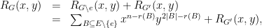
Although isolated nodes are immaterial for graphical 2-polymatroids, we augment them to include and . We replace by the signed node count and use its negative portion separately. By characterizing , the recipe theorem extends this representation even further:

Theorem 3 (Representation Theorem) For any G2PM with rank function ,

This says that is just an extension of from G2PMs to our augmented class of graphs. We give a fresh proof of the theorem.

Proof: For the completely empty graph, there is just the term and all exponents are zero, so the value is as required. For , we have the term for with (and ), which leaves . For , we have and also . The result is , again as required.

Because this is proving confluence, the only case of disjoint graphs we need to consider is adding one or . The above shows that the effect is to multiply by , or respectively, by . To save the case of recursing on below, we include that here: is just without adding the circle, whereas adds two , so the net effect is multiplying by , again as required.

This also lets us suppose that has no isolated nodes, so after all, and we may let be any member of . Again write for ; note that both and may have and/or . Consider subsets of that do not contain . Then Therefore when we begin the induction:

the first term already gives us the part of the sum in (3) that is over without . So we need only show that

Note that the edge set of can be identified with , even though some edges may become loops or circles. If is a loop then still has but . Thus we have by induction:

Equating (4) and (5) as formal polynomials gives the same necessary and sufficient condition on the powers of and :

This is true because always touches the one-or-two nodes that are exploded away, whereas does not touch them in (but touches everything else touches in ) and the difference is .

Combined with the recipe theorem we obtain the following, which re-emphasizes that for real is always a real polynomial:

Corollary 4 For any augmented G2PM with rank function , and all :

The Points

The quick finish to the proof of Theorem 3—combining what could be several cases of versus into one—can also be viewed through the lens of duality. Then the complement of in does not include , so is unchanged by removing . As we noted in the previous post, however, need not be the rank function of a graph. Thus the proof gives a handle on manipulating a wider class of structures via graph theory. It moreover seems extendable to all 2-polymatroids augmented with , so as to give extending .

The beauty of the recipe theorem is that a whole host of recursions become encoded by evaluations of the polynomials . As we noted with the Tutte polynomial and with the Oxley-Whittle polynomial , evaluations of them at certain points convey information about the graphs. For many points the information is -hard.

The case we care most about now is , . We showed how this evaluates the tractable subclass of quantum stabilizer circuits. This makes imaginary, but by Corollary 4 the values at real points are real.

When we have , so the value agrees with the polynomial in that post. The fact that evades the -hardness technique in the paper by Steve Noble which we also discussed there. So let us now abbreviate as . Then evaluates stabilizer circuits in polynomial time.

What other points are easy to evaluate, given ?

The point may even be nontrivial. If has no isolated nodes then the sum is over spanning edge-subsets and becomes

Is this in polynomial time?

Open Problems

What more can we gain from this augmentation and streamlining of Tutte-Grothendieck invariants? Can we find further characterizations of the polynomials and ? What can be done with -polymatroids with , which might allow evaluating more quantum circuits?

[some word improvements]