A Proof Of The Halting Theorem
Toward teaching computability and complexity simultaneously

|
| Large Numbers in Computing source |
Wilhelm Ackermann was a mathematician best known for work in constructive aspects of logic. The Ackermann function is named after him. It is used both in complexity theory and in data structure theory. That is a pretty neat combination.
I would like today to talk about a proof of the famous Halting Problem.
This term at Georgia Tech I am teaching CS4510, which is the introduction to complexity theory. We usually study general Turing machines and then use the famous Cantor Diagonal method to show that the Halting Problem is not computable. My students over the years have always had trouble with this proof. We have discussed this method multiple times: see here and here and here and in motion pictures here.
This leads always to the question, what really is a proof? The formal answer is that it is a derivation of a theorem statement in a sound and appropriate system of logic. But as reflected in our last two posts, such a proof might not help human understanding. The original meaning of “proof” in Latin was the same as “probe”—to test and explore. I mean “proof of the Halting Problem” in this sense. We think the best proofs are those that show a relationship between concepts that one might not have thought to juxtapose.
Diagonal and Impossible
The question is how best to convince students that there is no way to compute a halting function. We can define Turing machines 

How can we prove that 
Trying the diagonal method means first defining the set

We need to have already defined what “accept” means. OK, we show that there is no machine 


Ken in his classes goes the
It is impossible for a function
to give the value
—or any greater value.
Implementations of this, however, resort to double loops to define 
The Proof
Here is the plan. As usual we need to say that 

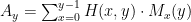
Now let
Theorem 1 The function
is not computable.
Proof: Define the function 

Suppose that 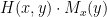


Now if the theorem is false, then there must be some 


This is impossible and so the theorem follows.

Extending Simplicity
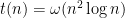
What Ken and I are really after is relating this to hierarchies in complexity classes. When the 


Ackermann’s famous function 
In complexity theory we have various time and space hierarchy theorems, say where ![{\mathsf{DTIME}[O(n^2)]}](https://s0.wp.com/latex.php?latex=%7B%5Cmathsf%7BDTIME%7D%5BO%28n%5E2%29%5D%7D&bg=ffffff&fg=000000&s=0&c=20201002)
![{\mathsf{C' = DTIME}[t(n)]}](https://s0.wp.com/latex.php?latex=%7B%5Cmathsf%7BC%27+%3D+DTIME%7D%5Bt%28n%29%5D%7D&bg=ffffff&fg=000000&s=0&c=20201002)


Suppose we’re happy with ![{\mathsf{C' = DTIME}[n^3]}](https://s0.wp.com/latex.php?latex=%7B%5Cmathsf%7BC%27+%3D+DTIME%7D%5Bn%5E3%5D%7D&bg=ffffff&fg=000000&s=0&c=20201002)


We’d like the “non-tight” proofs to be simple enough to combine with the above proof for halting. This leads into another change we’d like to see. Most textbooks define computability several chapters ahead of complexity, so the latter feels like a completely different topic. Why should this be so? It is easy to define the length and space usage of a computation in the same breath. Even when finite automata are included in the syllabus, why not present them as special cases of Turing machines and say they run in linear time, indeed time 
Open Problems
Is the above Halting Problem proof clearer than the usual ones? Or is it harder to follow?
What suggestions would you make for updating and tightening theory courses? Note some discussion in the comments to two other recent posts.
[some word fixes]


This is *way* less clear. I feel you hide the self-reference in the trick of summing up over all computations in a way that doesn’t easily generalize to other similar proofs.
The intuition one wants to convey with the halting problem is that: If the halting problem was computable we could define a computation that asks if that computation halts and does the opposite. I feel if you don’t get this across you might as well just assert it’s not computable since this is the essential trick used to prove any similar statement.
Yes, that proof goes through the fixed point theorem but I actually find that the fixed point theorem (or at least the part needed here) is super easy for modern students to grasp. OF COURSE a computation can scan through memory and read off it’s own source.
So take the program that reads it’s own `source’ off and then on input y runs H(‘source’, y)… then explain that this is all the fixed point theorem does in the formal version.
I agree, this feels like a tricky calculation that mysteriously works. I think that one thing you can rely on is that today students know (at least to some extent) how to code, how a simple computer program looks like. Instead of Turing machines, you can present the whole proof with C++!
typo: night should be might.
Thanks for comments from both.
The method used here does work in other cases by the way. Perhaps we should have spelled that out. Or will do that in the future. Separating classes by growth is a common tool. It is used for example with primitive recursive functions and in a proof of Paris-Harrington’s result.
Thanks
“Most textbooks define computability several chapters ahead of complexity, so the latter feels like a completely different topic. Why should this be so? It is easy to define the length and space usage of a computation in the same breath.”
Shameless plug: Stephan Mertens and I agree with you 🙂
Why not start (at least to give the students intuition) with a “software-level” proof: suppose that there is a subroutine Halt(P,x) that tells us, in finite time, whether or not a program P halts when given input on x. Then we could use it in the following program,
Catch22(P)
if Halts(P,P) then loop forever
else halt
and then ask what would happen if we ran Catch22(Catch22).
When I teach this stuff, I start by giving this proof. I then try to impress on the students that ideas like subroutines, universal programs that run other programs, and so on were hard-won — that people like Turing, Church, and Gödel had to do all this “from scratch”, using things like Gödel numbers instead the modern notion of source code. Their achievements are incredible, but we can honor them by using the high-level picture that they made possible.
We then talk about e.g. the time hierarchy theorem by noting that we _can_ solve the Halting problem for P, if we have an upper bound on P’s running time — if f(n)=o(g(n)), then we can solve the Halting Problem for programs that run in time f(n), using g(n) time to simulate them. But the very same argument shows that g(n) _needs_ to grow faster than f(n), and this shows that TIME(f(n)) is a proper subset of TIME(g(n)). To put it differently, any universal simulation of programs by other programs must have some overhead* — which is a lovely high-level conclusion to be able to draw.
*although not necessarily the log factor we get from Turing machines. For instance, in the RAM model the overhead can be a multiplicative constant.
It’s of no use to try to “better explain” Gödel incompleteness theorem, the Smoryński proof is among the simplest yet it is not “well received” (to say the least) to dismiss the Profound Metaphysical Problem of incompleteness (consciousness, AI, humans over machines, God, etc, etc…)
See my comment at Peter Smith’s blog Logic Matters. and the replies…
1. Is there no better picture of Ackermann anywhere? He lived until 1962 so there should be a more flattering one. (Sorry, bit of a hobby horse of mine. I posted on the math stackexchange without any results.)
2. Unlike others here, I teach undergrads solely and in this course feel that one of the main needs is to convey what the results are “really about”. It is great to bring in complexity, because that’s where it is at, right? But I don’t know that hiding the diagonalization, or at least making it less overt, helps with the “really.” (For what its worth, I do what Chris Moore does.)
I teach the Recursion Theorem as what happens when diagonalization fails and so at the moment I like having diagonalization be overt, although of course I could be convinced that the tradeoff is worth it.
Hi Jim. I totally agree with showing Cantor’s diagonalization (as well as Russell’s paradox, Berry’s, etc.) Then we can point out that if we have rows and columns corresponding to programs, calling Catch22(Catch22) goes along the diagonal, and the internal “if” of Catch22 provides the flip.
I always throw in some descriptions of snakes eating their own tails, Möbius strips, and so on…
Another diagonalization, which deserves to be taught more often (including at the undergrad level) is this:
Tweak(P)
..return P(P)+1 [or if you want a Boolean, not(P(P))]
with the understanding that (just as would happen if we tried to run this in real life) Tweak(P) never halts if P(P) never halts. If we run Tweak(Tweak) and it halts, it returns a value such that
P(P) = P(P)+1
The escape from this contradiction is that some programs never halt on some inputs (and indeed, Tweak(Tweak) is one of these). That is, some partial recursive functions are really partial: there’s no model of computation which 1) is universal in the sense of being able to run any program, and 2) which always halts.
Why is the partial sum A_y nonnegative? As far as I can see, nothing forbids M_x from returning negative integers.